Plot the Best-fit Model
The second step is to plot the best-fit model and make sure that the model
accurately reproduces the data. You can do this using
visualize.bestFit().
Some Preliminaries
Caution
You must run visualize.bestFit() from inside a CASA terminal OR you
must install MIRIAD and add the following line to config.yaml:
UseMiriad: True
Note
To run visualize.bestFit() from inside CASA, follow these steps
Install casa-python. This makes it easy to install custom python packages in CASA using pip.
Install
pyyamlandastropyinto your CASA python environment.
casa-pip install pyyamlcasa-pip install astropyInspect $HOME/.casa/init.py and ensure that it contains a link to the directory where
pyyamlandastropywere installed. In my case, the file already had the following:import site site.addsitedir(“/Users/rbussman/.casa/lib/python2.7/site-packages”)
So, I had to add the following lines:
site.addsitedir(“/Users/rbussman/.casa/lib/python/site-packages”) site.addsitedir(“/Users/rbussman/python/uvmcmcfit”)
This allowed CASA to recognize that
pyyamlanduvmcmcfitwere installed. You may have placeduvmcmcfitin a different directory, so modify these instructions accordingly.
Note
To install MIRIAD on Mac, try the MIRIAD MacPorts page
Caution
If you use MIRIAD to make images of the best-fit model, you must create a special cshell script called image.csh. This file should contain the instructions needed for MIRIAD to invert and deconvolve the simulated visibilities from the best-fit model.
The Simplest Best-fit Plot
Generating a simple plot of the best-fit model should be straightforward:
import visualize
visualize.bestFit()
If you run this routine in CASA, you will enter an interactive cleaning session.
Note
See this ALMA tutorial for help on interactive cleaning.
After the cleaning session finishes, two plots will be produced like the ones shown below.
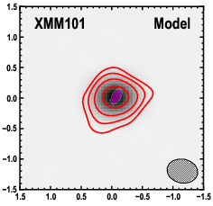
Left panel: ALMA 870um imaging of XMM101 (red contours, starting at
+/-3-sigma and increasing by factors of sqrt(2)) overlaid on the best-fit model
from uvmcmcfit (grayscale). The half-power shape of the source Source0
in this case, is shown by a magenta ellipse. The shape of the synthesized beam
is represented by the hatched black ellipse.
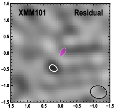
Right panel: Same as left panel, but showing the residual image after subtracting the best-fit model simulated visibilities from the observed visibilities. White and black contours trace positive and negative contours, respectively.
In this case, the model provides a good fit. There is evidence that the source is elongated in a direction perpendicular to the semi-major axis of the synthesized beam.
Comparison to Alternative Imaging
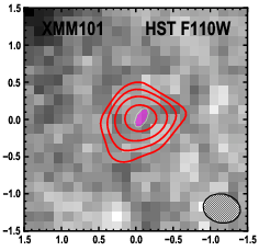
You can also compare the best-fit model to an image at an alternative wavelength (e.g., to compare lens properties with an optical or near-IR image of the lens). Do this by adding the following keyword:
visualize.bestFit(showOptical=True)
You should get the same results as above, but with an additional plot showing the comparison with the alternative image. Below is an example comparing the ALMA 870um imaging and best-fit model with HST F110W imaging.
Additional Options
You can turn off interactive cleaning in CASA:
visualize.bestFit(interactive=False)
visualize.bestFit() produces a large number of intermediate stage files
that are automatically deleted as the last step in the program. These can
sometimes be useful for debugging. To stop the program from automatically
deleting all intermediate files, use the following option:
visualize.bestFit(cleanup=False)